Clipping with Geometries

Author:

Howard Butler

Contact:

howard@hobu.co

Date:

11/09/2015

Introduction

This tutorial describes how to construct a pipeline that takes in geometries and clips out data with given geometry attributes. It is common to desire to cut or clip point cloud data with 2D geometries, often from auxiliary data sources such as OGR-readable Shapefiles. This tutorial describes how to construct a pipeline that takes in geometries and clips out point cloud data inside geometries with matching attributes.

Example Data

This tutorial utilizes the Autzen dataset. In addition to typical PDAL software (fetch it from Download), you will need to download the following two files:

• https://github.com/PDAL/data/autzen/autzen.laz

• https://github.com/PDAL/PDAL/raw/master/test/data/autzen/attributes.json

Stage Operations

This operation depends on two stages PDAL provides. The first is the filters.overlay stage, which allows you to assign point values based on polygons read from OGR. The second is filters.range, which allows you to keep or reject points from the set that match given criteria.

See also

filters.python allow you to construct sophisticated logic for keeping or rejecting points in a more expressive environment.

Data Preparation

Autzen Stadium, a 100 million+ point cloud file.

The data are mixed in two different coordinate systems. The LAZ file is in Oregon State Plane Ft. and the GeoJSON defining the polygons is in EPSG:4326. We have two options – project the point cloud into the coordinate system of the attribute polygons, or project the attribute polygons into the coordinate system of the points. The latter is preferable in this case because it will be less math and therefore less computation. To make it convenient, we can utilize OGR’s VRT capability to reproject the data for us on-the-fly:

<OGRVRTDataSource>
    <OGRVRTWarpedLayer>
        <OGRVRTLayer name="OGRGeoJSON">
            <SrcDataSource>attributes.json</SrcDataSource>
            <LayerSRS>EPSG:4326</LayerSRS>
        </OGRVRTLayer>
        <TargetSRS>+proj=lcc +lat_1=43 +lat_2=45.5 +lat_0=41.75 +lon_0=-120.5 +x_0=399999.9999999999 +y_0=0 +ellps=GRS80 +units=ft +no_defs</TargetSRS>
    </OGRVRTWarpedLayer>
</OGRVRTDataSource>

Note

The GeoJSON file does not have an externally-defined coordinate system, so we are explicitly setting one with the LayerSRS parameter. If your data does have coordinate system information, you don’t need to do that.

Save this VRT definition to a file, called attributes.vrt in the same location where you stored the autzen.laz and attributes.json files.

The attribute GeoJSON file has a couple of features with different attributes. For our scenario, we want to clip out the yellow-green polygon, marked number “5”, in the upper right hand corner.

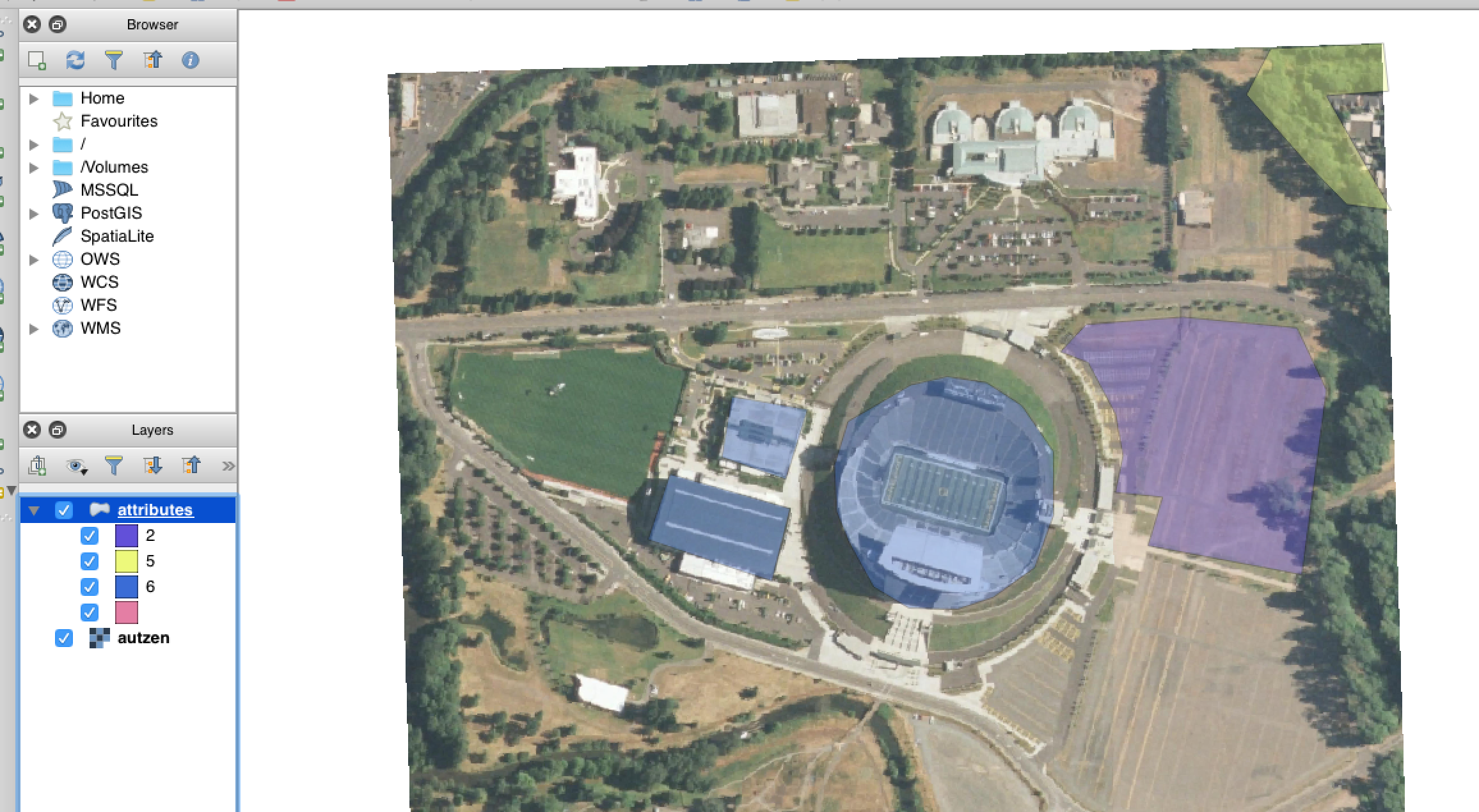
We want to clip out the polygon in the upper right hand corner. We can view the GeoJSON geometry using something like QGIS

Pipeline

A PDAL pipeline is how you define a set of actions to apply to data as they are read, filtered, and written.

[
    "autzen.laz",
    {
      "type":"filters.overlay",
      "dimension":"Classification",
      "datasource":"attributes.vrt",
      "layer":"OGRGeoJSON",
      "column":"CLS"
    },
    {
      "type":"filters.range",
      "limits":"Classification[5:5]"
    },
    "output.las"
]

• readers.las: Define a reader that can read ASPRS LAS or LASzip data.

• filters.overlay: Using the VRT we defined in Data Preparation, read attribute polygons out of the data source and assign the values from the CLS column to the Classification field.

• filters.range: Given that we have set the Classification values for the points that have coincident polygons to 2, 5, and 6, only keep Classification values in the range of 5:5. This functionally means we’re only keeping those points with a classification value of 5.

• writers.las: write our content out using an ASPRS LAS writer.

Note

You don’t have to use only Classification to set the attributes with filters.overlay. Any valid dimension name could work, but most LiDAR softwares will display categorical coloring for the Classification field, and we can leverage that behavior in this scenario.

Processing

1. Save the pipeline to a file called shape-clip.json in the same directory as your attributes.json and autzen.laz files.

2. Run pdal pipeline on the json file.

   $ pdal pipeline shape-clip.json
   

3. Visualize output.las in an environment capable of viewing it. http://plas.io or CloudCompare should do the trick.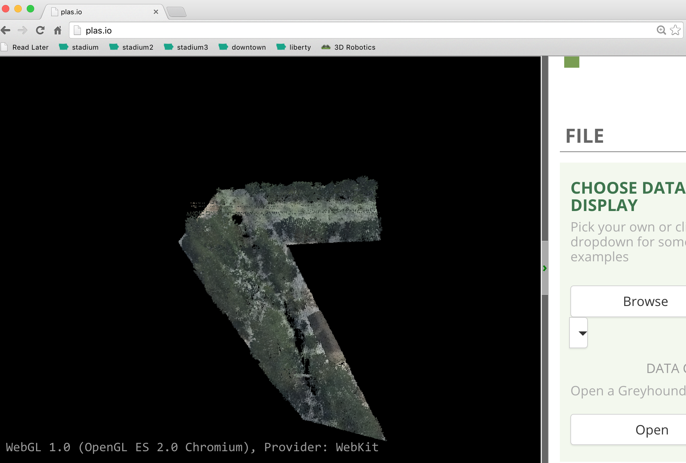

   

Conclusion

PDAL allows the composition of point cloud operations. This tutorial demonstrated how to use the filters.overlay and filters.range stages to clip points with shapefiles.