Colorizing points with imagery

This exercise uses PDAL to apply color information from a raster onto point data. Point cloud data, especially LiDAR, do not often have coincident color information. It is possible to project color information onto the points from an imagery source. This makes it convenient to see data in a larger context.

Exercise

PDAL provides a filter to apply color information from raster files onto point cloud data. Think of this operation as a top-down projection of RGB color values on the points.

Because this operation is somewhat complex, we are going to use a pipeline to define it.

{
    "pipeline": [
        "./exercises/analysis/thinning/uncompahgre.laz",
        {
            "type": "filters.colorization",
            "raster": "./exercises/analysis/colorization/casi-2015-04-29-weekly-mosaic.tif"
        },
        {
            "type": "filters.expression",
            "expression": "Red >= 1"
        },
        {
            "type": "writers.las",
            "compression": "true",
            "minor_version": "2",
            "dataformat_id": "3",
            "filename":"./exercises/analysis/colorization/uncompahgre-colored.laz"
        },
        {
            "type": "writers.copc",
            "filename": "./exercises/analysis/colorization/uncompahgre-colored.copc.laz",
            "forward": "all"
        }
    ]
}

Note

This JSON file is available in your workshop materials in the ./exercises/analysis/colorization/colorize.json file. Remember to open this file and replace each occurrence of ./ with the correct path for your machine.

Pipeline breakdown

1. Reader

After our pipeline errata, the first item we define in the pipeline is the point cloud file we’re going to read.

"./exercises/analysis/thinning/uncompahgre.laz",

2. filters.colorization

The filters.colorization PDAL filter does most of the work for this operation. We’re going to use the default data scaling options. This filter will create PDAL dimensions Red, Green, and Blue.

{
    "type": "filters.colorization",
    "raster": "./exercises/analysis/colorization/casi-2015-04-29-weekly-mosaic.tif"
},

3. filters.expression

A small challenge is the raster will colorize many points with NODATA values. We are going to use the filters.expression to filter keep any points that have Red >= 1.

{
    "type": "filters.expression",
    "expression": "Red >= 1"
},

4. writers.las

We could just define the uncompahgre-colored.laz filename, but we want to add a few options to have finer control over what is written. These include:

{
    "type": "writers.las",
    "compression": "true",
    "minor_version": "2",
    "dataformat_id": "3",
    "filename":"./exercises/colorization/analysis/uncompahgre-colored.laz"
}

1. compression: LASzip data is ~6x smaller than ASPRS LAS.

2. minor_version: We want to make sure to output LAS 1.2, which will provide the widest compatibility with other softwares that can consume LAS.

3. dataformat_id: Format 3 supports both time and color information

5. writers.copc

We will then turn the uncompahgre-colored.laz into a COPC file for vizualization with QGIS using the stage below.

{
    "type": "writers.copc",
    "filename": "./exercises/analysis/colorization/uncompahgre-colored.copc.laz"
    "forward": "all"
}

1. forward: List of header fields to be preserved from LAS input file. In this case, we want all fields to be preserved.

Note

writers.las and writers.copc provide a number of possible options to control how your LAS files are written.

Execution

Invoke the following command, substituting accordingly, in your Conda Shell:

$ pdal pipeline ./exercises/analysis/colorization/colorize.json

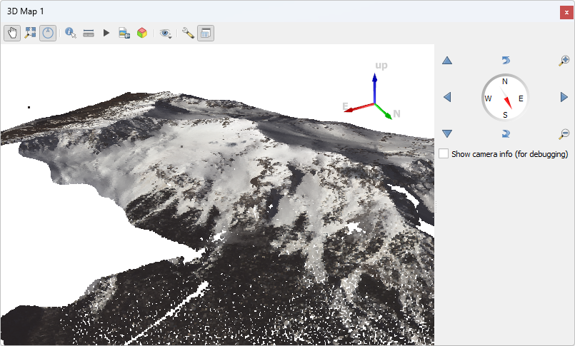
Visualization

Use one of the point cloud visualization tools you installed to take a look at your uncompahgre-colored.laz output. In the example below, we simply opened the file using QGIS.

Notes

1. Applying color information that is not time-coincident with the point cloud data will mean you will see discontinuities.

2. GDAL is used to read the image source. Any GDAL-readable data format can be used.

3. There are performance considerations to be aware of depending on the raster format and type being used. See filters.colorization for more information.

4. These data are of Uncompahgre Basin courtesy of the NASA Airborne Snow Observatory.