Removing noise

This exercise uses PDAL to remove unwanted noise in an airborne LiDAR collection.

Exercise

PDAL provides the outlier filter to apply a statistical filter to data.

Because this operation is somewhat complex, we are going to use a pipeline to define it.

{
    "pipeline": [
        "./exercises/analysis/denoising/18TWK820985.laz",
        {
            "type": "filters.outlier",
            "method": "statistical",
            "multiplier": 3,
            "mean_k": 8
        },
        {
            "type": "filters.expression",
            "expression": "(Classification != 7) && (Z >= -100 && Z <= 3000)"
        },
        {
            "type": "writers.las",
            "compression": "true",
            "minor_version": "2",
            "dataformat_id": "0",
            "filename":"./exercises/analysis/denoising/clean.laz"
        },
        {
            "type": "writers.copc",
            "filename": "./exercises/analysis/denoising/clean.copc.laz",
            "forward": "all"
        }
    ]
}

Note

This pipeline is available in your workshop materials in the ./exercises/analysis/denoising/denoise.json file.

Pipeline breakdown

1. Reader

After our pipeline errata, the first item we define in the pipeline is the point cloud file we’re going to read.

"./exercises/analysis/denoising/18TWK820985.laz",

2. filters.outlier

The PDAL outlier filter does most of the work for this operation.

{
    "type": "filters.outlier",
    "method": "statistical",
    "multiplier": 3,
    "mean_k": 8
},

3. filters.expression

At this point, the outliers have been classified per the LAS specification as low/noise points with a classification value of 7. The range filter can remove these noise points by constructing a range with the value Classification != 7, which passes every point with a Classification value not equal to 7.

Even with the filters.outlier operation, there is still a cluster of points with extremely negative Z values. These are some artifact or mis-computation of processing, and we don’t want these points. We can construct another range to keep only points that are within the range \(-100 <= Z <= 3000\).

Both ranges are passed as a AND-separated list to the expression based range filter via the expression option.

{
    "type": "filters.expression",
    "expression": "Classification != 7 && (Z >= -100 && Z <= 3000)"
},

4. writers.las

We could just define the clean.laz filename, but we want to add a few options to have finer control over what is written. These include:

{
    "type": "writers.las",
    "compression": "true",
    "minor_version": "2",
    "dataformat_id": "0",
    "filename":"./exercises/analysis/denoising/clean.laz"
}

1. compression: LASzip data is ~6x smaller than ASPRS LAS.

2. minor_version: We want to make sure to output LAS 1.2, which will provide the widest compatibility with other softwares that can consume LAS.

3. dataformat_id: Format 0 supports both time and color information

5. writers.copc

We will then turn the clean.laz file into a COPC file for vizualization with QGIS using the stage below.

{
    "type": "writers.copc",
    "filename": "./exercises/analysis/colorization/clean.copc.laz"
    "forward": "all"
}

1. forward: List of header fields to be preserved from LAS input file. In this case, we want all fields to be preserved.

Note

writers.las and writers.copc provide a number of possible options to control how your LAS files are written.

Execution

Invoke the following command, substituting accordingly, in your ` Shell`:

$ pdal pipeline ./exercises/analysis/denoising/denoise.json

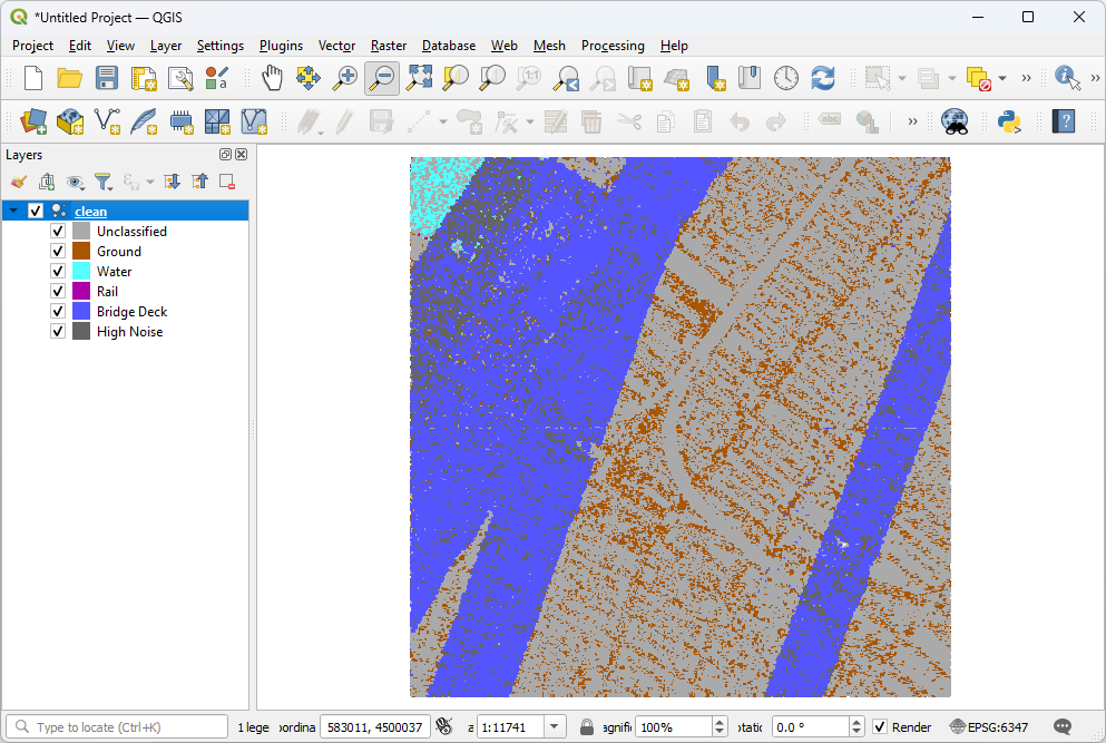
Visualization

Use one of the point cloud visualization tools you installed to take a look at your clean.copc.laz output. In the example below, we simply opened the file using QGIS.

Notes

1. Control the aggressiveness of the algorithm with the mean_k parameter.

2. filters.outlier requires the entire set in memory to process. If you have really large files, you are going to need to split them in some way.