Visualizing acquisition density
This exercise uses PDAL to generate a density surface. You can use this surface to summarize acquisition quality.
Exercise
PDAL provides an application to compute a vector field of hexagons computed with filters.hexbin. It is a kind of simple interpolation, which we will use for visualization in QGIS.
Command
Invoke the following command, substituting accordingly, in your Shell:
$ pdal density ./exercises/analysis/density/uncompahgre.laz  \
-o ./exercises/analysis/density/density.sqlite \
-f SQLite
> pdal density ./exercises/analysis/density/uncompahgre.laz  ^
-o ./exercises/analysis/density/density.sqlite ^
-f SQLite
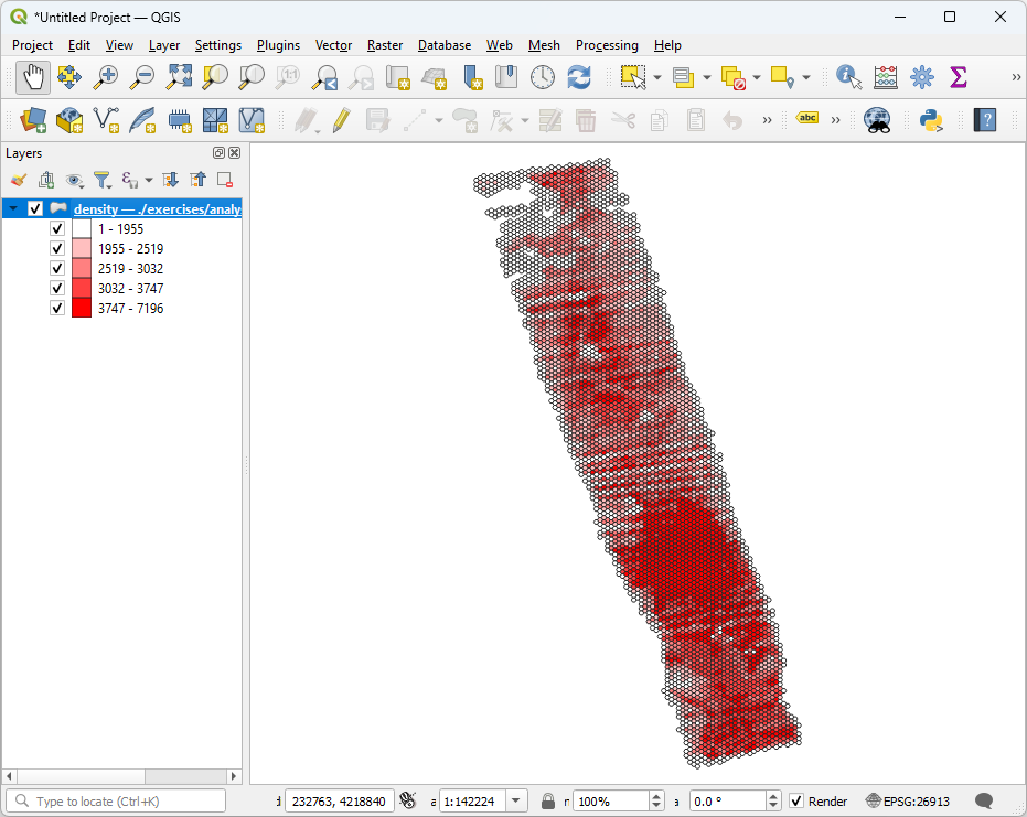
Visualization
The command uses GDAL to output a SQLite file containing hexagon polygons. We will now use QGIS to visualize them.
Add a vector layer
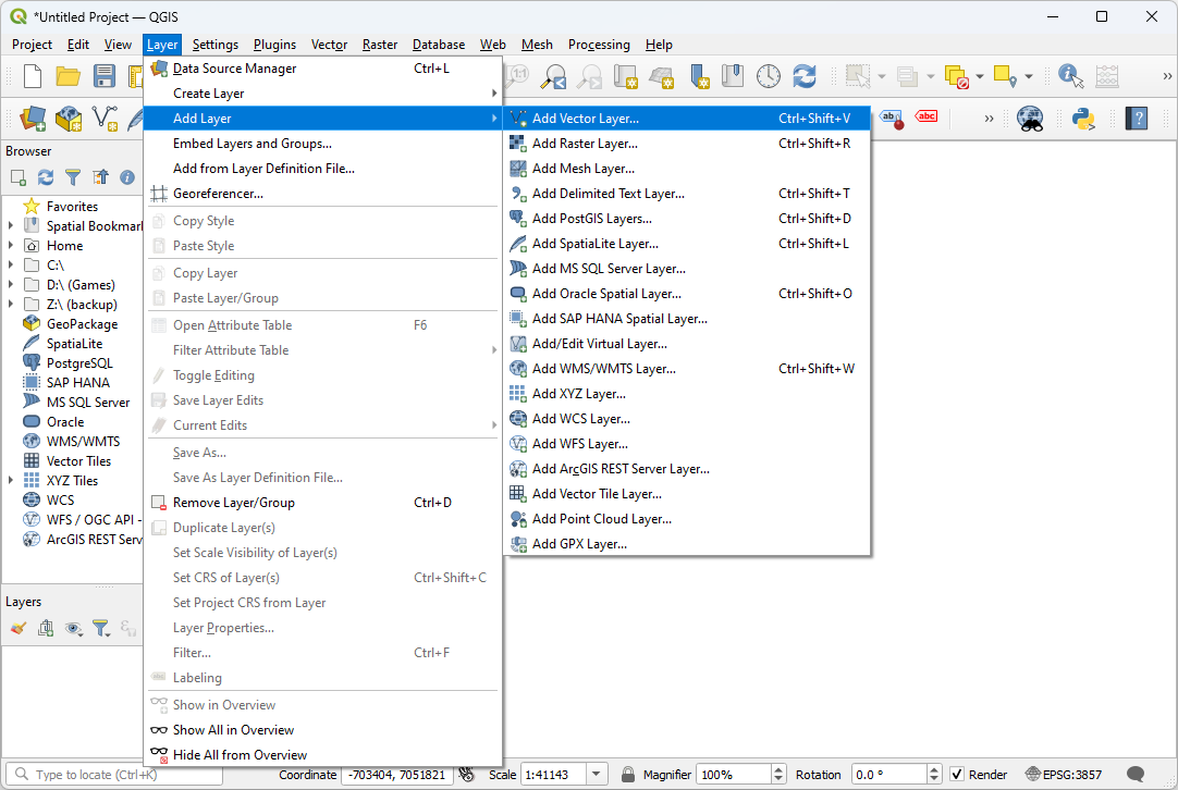
Navigate to the output directory
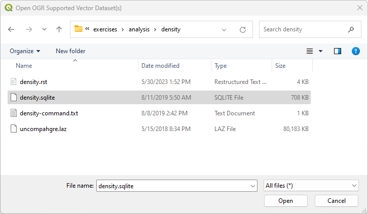
Add the
density.sqlitefile to the view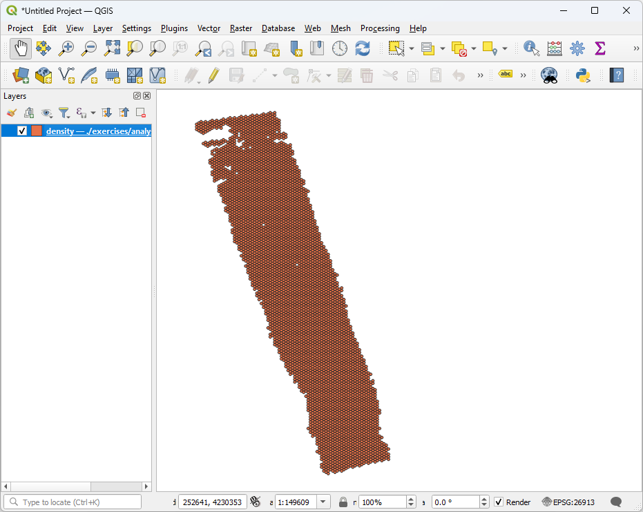
Right click on the
density.sqlitelayer in the Layers panel and then chooseProperties.Within the
Symbologytab, changeSingle SymboltoGraduatedin the drop down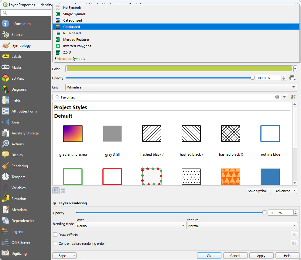
Choose the
Countcolumn to visualize
Choose the
Classifybutton to add intervals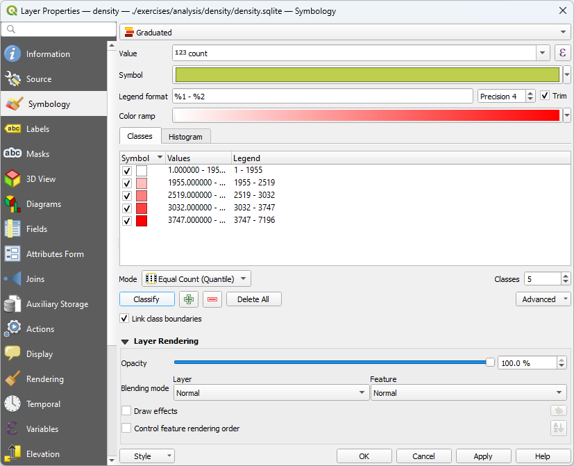
Adjust the visualization as desired

Notes
You can control how the density hexagon surface is created by using the options in filters.hexbin.
The following settings will use a hexagon edge size of 24 units.
--filters.hexbin.edge_size=24