Clipping data with polygons

This exercise uses PDAL to apply to clip data with polygon geometries.

Note

This exercise is an adaption of the PDAL tutorial.

Exercise

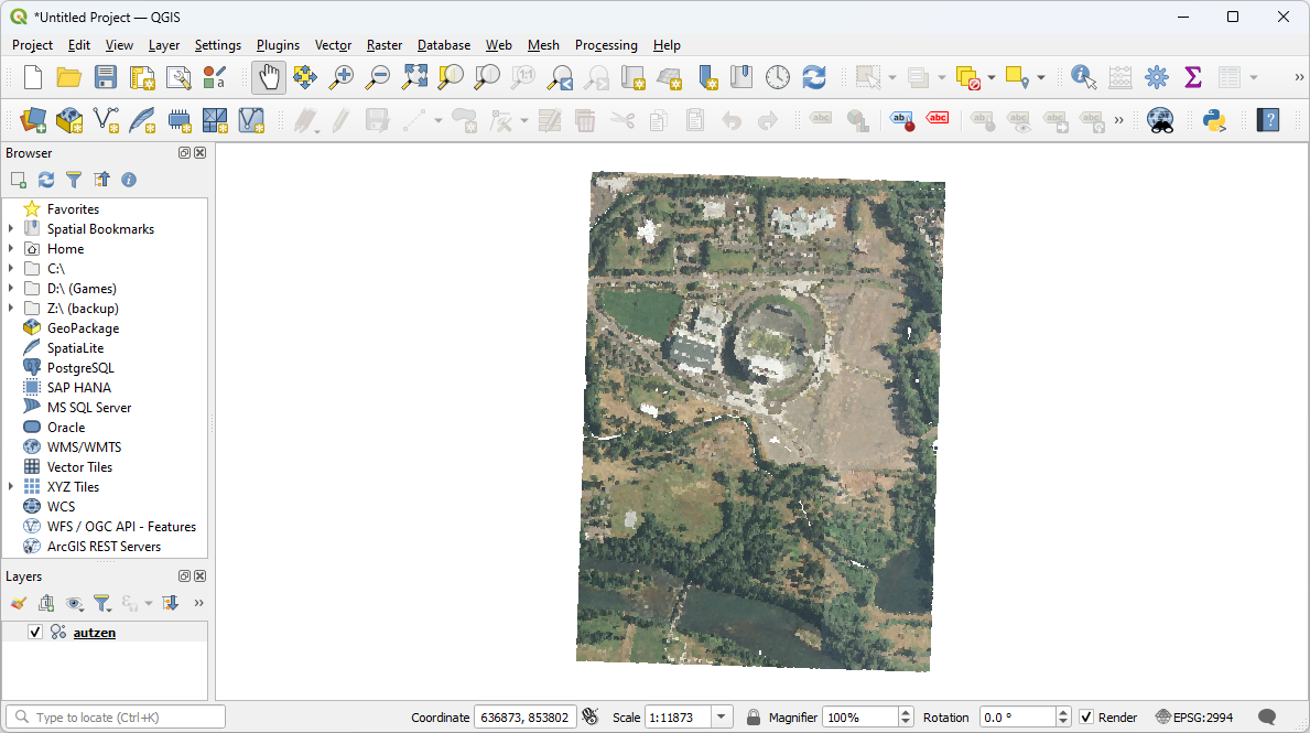
The autzen.laz file is a staple in PDAL and libLAS examples. You can download this file here and move it to ./exercises/analysis/clipping in your drive. We will use this file to demonstrate clipping points with a geometry. We’re going to clip out the stadium into a new COPC file.

Data preparation

The data are mixed in two different coordinate systems. The LAZ file is in Oregon State Plane Ft. and the GeoJSON defining the polygons, attributes.json, is in EPSG:4326. We have two options – project the point cloud into the coordinate system of the attribute polygons, or project the attribute polygons into the coordinate system of the points. The latter is preferable in this case because it will be less math and therefore less computation. To make it convenient, we can utilize OGR’s VRT capability to reproject the data for us on-the-fly:

<OGRVRTDataSource>
    <OGRVRTWarpedLayer>
        <OGRVRTLayer name="OGRGeoJSON">
            <SrcDataSource>./exercises/analysis/clipping/attributes.json</SrcDataSource>
            <SrcLayer>attributes</SrcLayer>
            <LayerSRS>EPSG:4326</LayerSRS>
        </OGRVRTLayer>
        <TargetSRS>+proj=lcc +lat_1=43 +lat_2=45.5 +lat_0=41.75 +lon_0=-120.5 +x_0=399999.9999999999 +y_0=0 +ellps=GRS80 +units=ft +no_defs</TargetSRS>
    </OGRVRTWarpedLayer>
</OGRVRTDataSource>

Note

This VRT file is available in your workshop materials in the ./exercises/analysis/clipping/attributes.vrt file. You will need to open this file, go to line 4 and replace ./ with the correct path for your machine.

A GDAL or OGR VRT is a kind of “virtual” data source definition type that combines a definition of data and a processing operation into a single, readable data stream.

Overlaying Attributes

To add our attributes.vrt file, perform the following:

1. In QGIS, select Layer -> Add Layer -> Add Vector Layer

2. Add attributes.vrt as the Vector Layer

3. Right click the new layer and select properties

4. Under “Symbology” on the left, select “categorized” from the drop-down

5. Change value from $id to cls

6. Below, select “Classify” and confirm

7. In the “Layer Rendering” drop-down, set “Opacity” to 50%

8. On the left, select “Labels”. Set the drop-down to “Single Labels”

9. Change value from id to cls and select “OK” on the bottom right

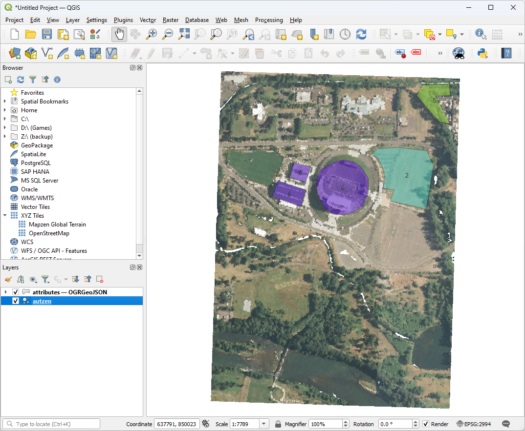
Note

Notice the numbers on the buildings and trees. These are the classifations given in the LIDAR Point Classes or LAS Specification. You can sort and single out these in JSON filters. ex. "expression": "Classification >= 3 && Classification <= 4" which only shows classes 3 to 4 which are medium and high vegetation.

ASPRS Standard LiDAR Point Classes (Point Data Record Format 0-5)

Classification Value (bits 0:4)	Meaning
0	Created, never classified
1	Unclassified
2	Ground
3	Low Vegetation
4	Medium Vegetation
5	High Vegetation
6	Building
7	Low Point (noise)
8	Model Key-point (mass point)
9	Water
10	Reserved for ASPRS Definition
11	Reserved for ASPRS Definition
12	Overlap Points
13-31	Reserved for ASPRS Definition

Note

The GeoJSON file does not have an externally-defined coordinate system, so we are explicitly setting one with the LayerSRS parameter. If your data does have coordinate system information, you don’t need to do that. See the OGR VRT documentation for more details.

Pipeline breakdown

{
    "pipeline": [
        "./exercises/analysis/clipping/autzen.laz",
        {
            "column": "CLS",
            "datasource": "./exercises/analysis/clipping/attributes.vrt",
            "dimension": "Classification",
            "layer": "OGRGeoJSON",
            "type": "filters.overlay"
        },
        {
            "expression": "Classification == 6",
            "type": "filters.expression"
        },
        {
            "type": "writers.copc",
            "filename": "./exercises/analysis/clipping/stadium.copc.laz",
            "forward": "all"
        }
    ]
}

Note

This pipeline is available in your workshop materials in the ./exercises/analysis/clipping/clipping.json file. Remember to replace each of the three occurrences of ./ in this file with the correct location for your machine.

1. Reader

autzen.laz is the LASzip file we will clip.

2. filters.overlay

The filters.overlay filter allows you to assign values for coincident polygons. Using the VRT we defined in Data preparation, filters.overlay will assign the values from the CLS column to the Classification field.

3. filters.expression

The attributes in the attributes.json file include polygons with values 2, 5, and 6. We will use filters.expression to keep points with Classification values in the range of 6:6.

4. Writer

We will write our content back out using a writers.las.

Execution

Invoke the following command, substituting accordingly, in your Conda Shell:

The –nostream option disables stream mode. The point-in-polygon check (see notes) performs poorly in stream mode currently.

$ pdal pipeline ./exercises/analysis/clipping/clipping.json --nostream

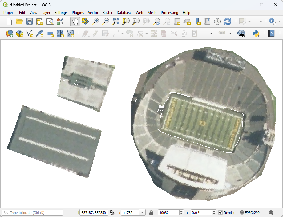
Visualization

Use one of the point cloud visualization tools you installed to take a look at your ./exercises/analysis/clipping/stadium.copc.laz output. In the example below, we opened the file to view it using QGIS.

Notes

1. filters.overlay does point-in-polygon checks against every point that is read.

2. Points that are on the boundary are included.